Meta'Omics Upgrade

Expanding the project from my metagenomics class has been on my to-do list for some time, but the older code needed an update first.

I’ve heard that if you don’t cringe at your old code, you haven’t been learning. I’ll start off by saying that returning to this project showed me just how far I’ve come in the eighteen months since I turned it in. In fairness to past me, I was under some serious time constraints. Despite all my professors promising that there was an abundance of biological data available for analysis, it still took days of research for me to even find a usable dataset. This, in addition to working retail in December and all the other end of semester tasks meant that I was prioritizing function, no matter how poor, over all other considerations. One lesson learned at the time was to email the authors of a potential dataset immediately. Biologists seem to have trouble providing relevant metadata with their datasets, but every scientist I’ve talked to has happily shared papers and data in the past.

The first improvement I made was to parallelize the dataset assembly. I really should have looked into this at the time, but I had never worked with so much data before. I had access to a cloud computing account through my class, and figured that having several machines processing different parts of the program would enough. However, simply adding a few lines from Concurrent Futures reduced the run time from many hours to just a few minutes. I also added a progress bar from TQDM and a bell sound clip so my scripts can share feedback features with my microwave.

The second upgrade was to make the move to a Jupyter Notebook. The original scripts had used a series of Argparse flags to trigger different routines, but I was still recording observations and run commands in a separate file. Like a notebook. Like parallelization, Jupyter Notebooks were a technology I had been vaguely aware of, but wasn’t sure I could spare the bandwidth to learn. Having now used it, I am a huge fan of being able to merge my code and observations together in the same document. Being able to output charts in-line with all my other notes is probably the best quality of life improvement a scientific programmer could ask for. I don’t know how many others missed the Jupyter train like I did, but it’s my new favorite tool.

This brings me to the improvements made to the project itself. The original idea was to see what kind of differences can be found in the functional profiles of meta’omic samples for different diseases. I realize that sentence was a lot, so let’s break it down.

‘Omics refers to the study of information content a biological system, and meta’omics refers to the total of a particular system within a given environment. For example, genomics is the study of the genome, and metagenomics is the study of all of the genomes present in a nasal swab, or a drop of pond water, or whatever. A functional profile is, appropriately enough, the total of set of functions contained within an ‘ome or meta’ome. Since protein function is tied directly to it’s structure, and since it’s structure can be imputed from the protein’s encoding in a nucleic acid, it is possible to assemble the total functional profile of a sample, even if many of those functions were not active when the sample was taken.

The difference in functional activity over time is the major difference between the metagenome and the metatranscriptome. The metagenome includes everything encoded in the DNA in the sample, meaning that it includes the total potential functional profile of every organism present. The metatranscriptome, on the other hand, comprises all of the RNA from the sample. Since RNA is the first molecule produced when a gene is active, the functional profile of a metatranscriptome only contains those functions that were active when the sample was taken (more accurately, in the time between sampling and sequencing, but that’s just a limitation of transcriptome data in general). The difference in functional profile in each data type boils down to the metagenome containing information on what a community could be doing, while the metatranscriptome shows what that community is up to right now.

The correlation between certain microbe community compositions and many diseases has been known for some time but, at least as of the start of this project, few if any studies existed that linked the functional profiles of microbe community disease. This surprised me, since bacteria commonly share genes, and therefore functional changes across species. The whole idea of species kind of breaks down when individuals both reproduce by fission and share genetic material asexually, and considering that members of the same apparent species can have radically different functional profiles, is of limited use when trying to figure out what the critters are up to.

My idea was to try to find out which of either metagenomic or metatranscriptomic data was more useful for determining the disease status of a sample, and how that compared to the same analysis using operational taxonomic units (species). I expected the results to vary by disease, since a condition caused by intermittent activation of a few functions would probably be best identified by metagenomic data, while metatranscriptomic data might show a stronger signal for a condition caused by the constant activity of a certain function. The specific outcomes of the experiment are contained in the paper I submitted, but as mentioned earlier, I only found a dataset for one disease, and it wasn’t functionally annotated.

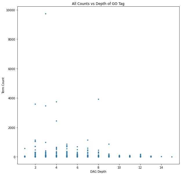
In order to get functional annotations, I needed to map the protein families used in the original project to their associated Gene Ontology (GO) terms. An ontology is a controlled and structured vocabulary used for making detailed descriptions and logical statements about a specific domain, and the GO is used for describing the function of genes. The features on the original dataset were protein families, and the samples were represented as the percent composition of each family. My first step was to collect all protein families present in my dataset and query the UniProt database for their GO annotations. The protein families were UniProt Reference Clusters (UniRef) defined by sharing 90% sequence identity with a representative protein. The UniRef families themselves didn’t have any GO annotations, so I used the representative proteins instead. Starting from 60,180 known protein families, 34,402 representative proteins had GO annotations containing at least one of 3,417 unique GO terms.

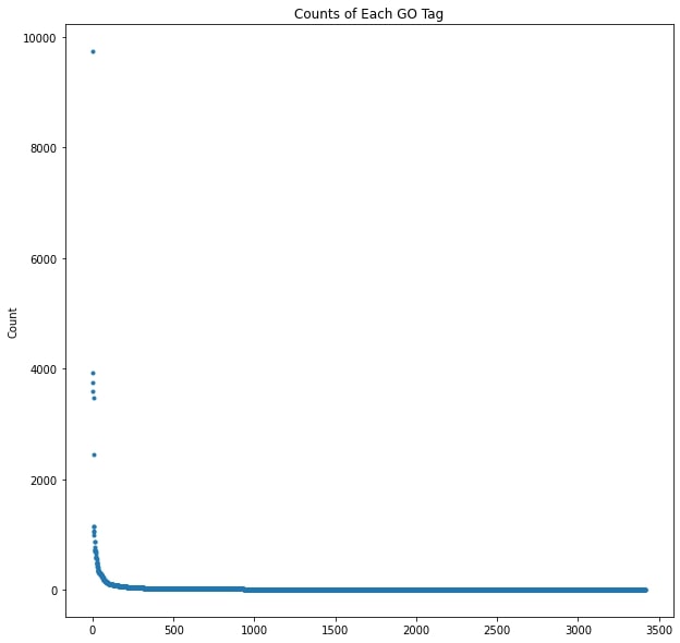
The overwhelming majority of the GO terms only occurred a handful of times, and the most common terms referred to critical cellular processes like “DNA binding” and “hydrolase activity.” The most common annotation, all the way up in the top left corner of the graph, is a high level term referring to “integral component of membrane.” That high level and common terms would be the most abundant wasn’t surprising, but there also wasn’t a visible correlation between the depth, and therefore specificity of a term and it’s frequency among the annotated proteins. There are clearly more terms with lower frequency, and a slight skew toward shallower depth, but there are many outliers along both axes.

The next step was to map the GO terms back to the datasets themselves. The protein families are unevenly distributed between the metagenome and metatranscriptome samples, and the specific families depend on the methods used to construct the different datasets. Each protein family was replaced with all of it’s GO annotations, with duplicate terms being summed together. Unannotated families were dropped altogether. In general, each dataset lost about 40% of it’s features when the unannotated protein families were dropped and another 40% reduction occurred when duplicate terms were combined. Since I had been adding percent composition values together when protein families shared a term, I also standardized the data.

I had used an array of machine learning models as a proxy for determining the information content of a sample. I figured that if a model had an easier time classifying the samples, I could try to identify the most important factors later. To compare the GO annotations to the original protein families, I converted the smallest metatranscriptome dataset to GO terms, trained a random forest classifier, and checked the classification accuracy. The result was the same, about 80% correct classification. Clearly there are still improvements to be made.

To start with, I know that the percentage of correct classification is not a good measure of machine learning accuracy. I was careful to control the sizes of each dataset, but I will be replacing the scoring metric with an ROC curve the next time I touch this project. Another basic improvement is to find more data, as my datasets are relatively small, and I need at least as many samples for a whole different disease to even start to answer my original question.

Finally, I need a smarter way of selecting my features. I would like to keep the relative abundance of each GO term, but just pooling the percent composition value from the protein family seems like a crude way to do it. I could try to standardize each term individually, but I could also see what happens when all that matters is the presence or absence of a term. There is no guarantee that the effect of a disease factor is correlated with it’s relative abundance after all. Another strategy could be to exclude the most common GO terms entirely, or to only use the most specific term associated with a gene family. The last, and probably best possibility is to perform a simple enrichment analysis rather than this roundabout machine learning proxy strategy. I’ve been reading up on the details of the GO in The Gene Ontology Handbook by Dessimoz and Škunca, and should have a few new ideas by the end as well. Between more data and smarter analysis, this project has a long way to go, but it should also be interesting and informative at every stage.